Binomial distribution (Intro to statistics)

1. Let us start with the definition of a function to simulate the tossing of a coin.

sim_binom<- function(how_many_tosses, how_many_samples){
results <- c()
heads_or_tails <- c(1, 2)
for(i in 1:how_many_samples){
  tosses <- sample(heads_or_tails, how_many_tosses, replace = TRUE)
  count <- 0
  for(j in tosses){
    if(j == 1){
    count = count+1
    }
  results[i] <- count/how_many_tosses
  }
}
return(hist(results, breaks = c(50)))
}

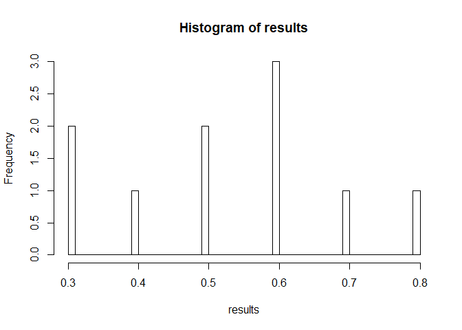
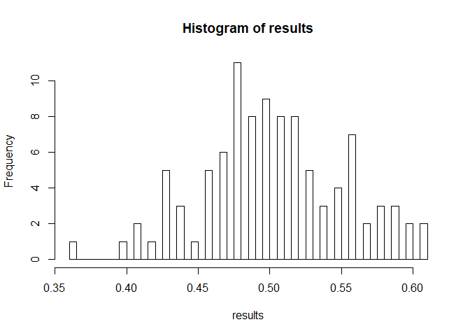
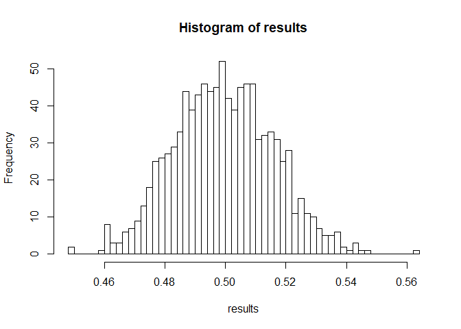
2. The simulations below will toss a fair coin N number of times and calculate the percentage of heads that appeared in our simulation. This process will be repeated X times.

sim_binom(10, 10) #Throwing the coin 10 times, and repeating the process 10 times.

sim_binom(100, 100) #Throwing the coin 100 times, and repeating the process 100 times.

sim_binom(1000, 1000) #Throwing the coin 1000 times, and repeating the process 1000 times.

3. Just a little help interpreting the histograms

The x axis indicates the percentage of heads that you got from tossing the coin N times. The Y axis represents how many times this event occurred. For instance, running the last simulation above, you will probably see that in ‘most’ of the cases you get something around 50% of heads and 50% of tails, which is expected from a fair coin.

4. Compare each one of the three simulations above and answer the following questions:

5. As the number of tosses increases, what do you observe from the #histogram?

6. For the last simulation with 1000 tosses, where are most cases centered at?

7. Does the shape of the histogram remind you of any distribution we have studied so far? Which one and why?

##Section 2

1. Imagine we do not have a fair coin and we want to calculate the probability of gettig exactly 2 heads out of 6 tosses.

p_of_heads = 0.7
p_of_tails = 0.3

2. There are many possibilities for getting 2 heads out of 6 tosses (e.g. HHTTTT, HTHTTT…). The probability of only one of these cases ocurring is:

prob <- (p_of_heads^2) * (p_of_tails^4)

3. But we have to multiply it by the number of times it can happen by tossing the coin 6 times. We calculate this by applying the combinatorial formula below:

combinatorial_possibilities = factorial(6) / (factorial(2)*factorial(4))

4. Now answering the questions: what is the probability of getting 2 successess in 6 attempts? Our final answer would be:

combinatorial_possibilities*prob

5. Try this one by yourself:

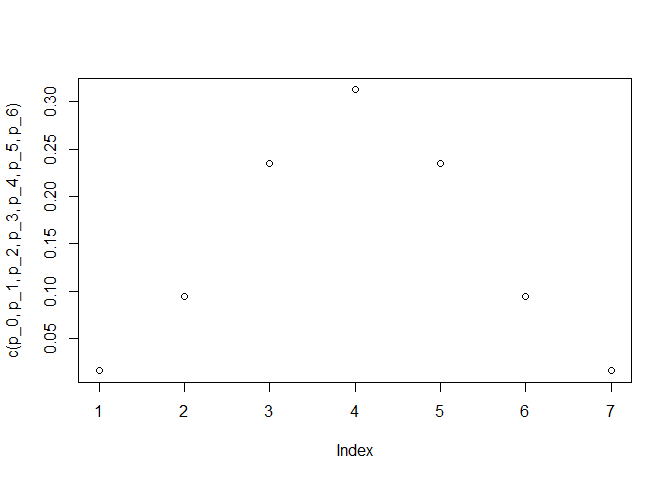
6. A basketball player has a 50% chance of scoring a point. If he throws the ball 6 times, what is the probability that he will get exactly 0, 1, 2, 3, 4, 5 and 6 points?

7. Before calculating, let R help us a little bit and let us define a function for calculating the probabilities:

binomial_calculator <- function(number_of_throws, p_win, p_lose, number_of_wins){
  prob <- (p_win^number_of_wins) * (p_lose^(number_of_throws-number_of_wins))
  combinatorial_possibilities = factorial(number_of_throws) / ( factorial(number_of_wins)*factorial((number_of_throws-number_of_wins)) )
  probability = combinatorial_possibilities*prob
  return(probability)
}

8. Calculating responses:

p_0 = binomial_calculator(6, 0.5, 0.5, 0) #0
p_1 = binomial_calculator(6, 0.5, 0.5, 1) #1
p_2 = binomial_calculator(6, 0.5, 0.5, 2) #2
p_3 = binomial_calculator(6, 0.5, 0.5, 3) #3
p_4 = binomial_calculator(6, 0.5, 0.5, 4) #4
p_5 = binomial_calculator(6, 0.5, 0.5, 5) #5
p_6 = binomial_calculator(6, 0.5, 0.5, 6) #6

9. Here is how we can interpret it: If the basketball player had an equal probability of missing and losing, by throwing a ball 6 times, we would expect him to get exactly 4 points (theoretically speaking). And the more he departed from this number of points, the more we would think that he does not have a 50% chance of missing. For instance, the probability of him getting exactly 0 points out of 6 throws, assuming an equal probability of scoring, would be as low as:

p_0

## [1] 0.015625

10. Now let us visualize what these probabilities look like:

plot(c(p_0, p_1, p_2, p_3, p_4, p_5, p_6))

11. Again, does this plot remind you of any distribution? Which one and why?

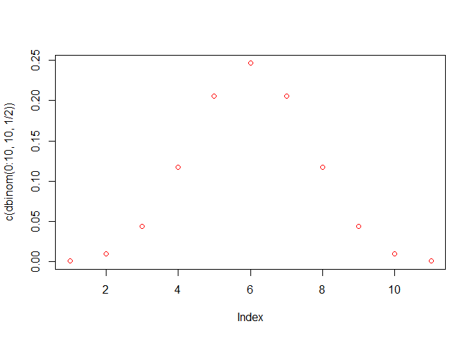
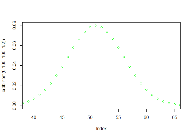
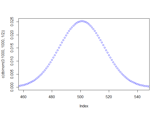
12. The plots below are showing you the probabilities of getting any number of heads from 0 to 10, 100, and 1000, assuming that we flipped a fair coin. It basically does the same thing we did before, but with larger sample sizes.

plot( c(dbinom(0:10, 10, 1/2)), col = 'red' )

plot( c(dbinom(0:100, 100, 1/2)), col = 'green', xlim = c(39, 65))

plot( c(dbinom(0:1000, 1000, 1/2)), col = 'blue',  xlim = c(460, 545))

13. Does that make sense to you? Look at the first graph and answer: *Why is it less probable to get 1 head out of 10 tosses than getting 5 heads out of 10 tosses?