Musicology on R
Pedro A. S. O. Neto
Major versus minor songs
Here I am conducting an illustratory study where I look for differences between major and minor songs.
Data set
I used Spotify’s web API to build a database consisting of 5820 albums and 78178 tracks. Each track is divided into several segments, and these segments are described in terms of loudness, energy, valence, danceability, and tempo. Details about how these variables were calculated are described here. The query and the API calls were written in Python, and are also available here.
1. Global analysis
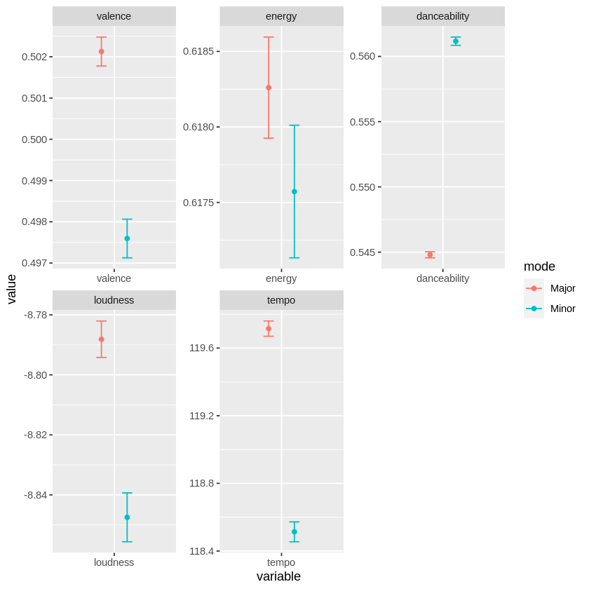
First, I computed mean and S.E.M for each one of our variables, collapsing across all tracks in our dataset. As expected, I found that major tracks tend to be higher in loudness, valence and tempo. Danceability, however, behaved differently from the other variables, as you can see in the graph below.
options(warn=-1); require("data.table"); require("ggplot2"); data <- fread("data2.csv")

se <- function(x) { return(sd(x, na.rm = T)/sqrt(length(x))) }
global <- plyr::ddply(data, c("mode"), dplyr::summarise,
                   valence = mean(valence, na.rm = TRUE),
                   energy = mean(energy, na.rm = TRUE),
                   danceability = mean(danceability, na.rm = TRUE),
                   loudness = mean(loudness_x, na.rm = TRUE),
                   tempo = mean(tempo_y, na.rm = TRUE))

global_se <- plyr::ddply(data, c("mode"), dplyr::summarise,
                   valence = se(valence),
                   energy = se(energy),
                   danceability = se(danceability),
                   loudness = se(loudness_x),
                   tempo = se(tempo_y))

global = melt(as.data.table(global)); global_se = melt(as.data.table(global_se))
global$se <- global_se$value

ggplot(global, aes(x = variable, y = value, color = mode))+
       facet_wrap(~variable, scale = 'free')+
       geom_point(position = position_dodge(width = 0.5), size = 1.5)+
       geom_errorbar(aes(ymin = value-se, ymax = value+se), position = position_dodge(width = 0.5), width = 0.2)

2. Analysis by segment
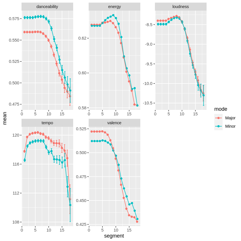
Next, I conducted the same analysis, but separating between segments of each track. The number of segments per track varied to a significant extent. For instance, whereas all tracks from the dataset had the first segment, only a small fraction of these tracks had a 150th segment.
In order to identify and exclude tracks with unusual number of segmentations, I conducted an outlier analysis based on interquantile ranges.
#Function returns a 0 tag indicating that the track is an outlier.
out_detector = function(s){
        li = quantile(s)[2] - IQR(s)*1.5; ls = quantile(s)[4] + IQR(s)*1.5; f = c()
        for(i in 1:length(s)){
            if( (s[i] > li) && (s[i] < ls)) {   f[[i]] = s[i]   }
            if(s[i] <= li)                  {   f[[i]] = 0  }
            if(s[i] >= ls)                  {   f[[i]] = 0 }}
            return(f)
        }

#Identify number of segments for each track
data <- data[order(track_number), max_seg := max(segment), by = track_id]

#Apply outlier tag
data$out_filter <- out_detector(data$max_seg)

#Filter tracks with many or few segments
data <- dplyr::filter(data, data$out_filter != 0)
After outlier exclusion, the average number of segmentation per track was approximatelly 6 (M = 5.86, SD = 3.51).
Results are displayed below. Overall, we see a trend of larger valence, loudness and tempo for major tracks. However, this pattern weakens towards the last segments of each track.
#Getting descriptives by segment of each track and mode
valence <- plyr::ddply(data, c("segment", "mode"), dplyr::summarise,
                   valence = mean(valence, na.rm = TRUE), se = se(valence))

energy <- plyr::ddply(data, c("segment", "mode"), dplyr::summarise,
                   energy = mean(energy, na.rm = TRUE), se = se(energy))

danceability <- plyr::ddply(data, c("segment", "mode"), dplyr::summarise,
                   danceability = mean(danceability, na.rm = TRUE), se = se(energy))

loudness <- plyr::ddply(data, c("segment", "mode"), dplyr::summarise,
                   loudness = mean(loudness_x, na.rm = TRUE), se = se(loudness_x))

tempo <- plyr::ddply(data, c("segment", "mode"), dplyr::summarise,
                   tempo = mean(tempo_y, na.rm = TRUE), se = se(tempo_y))

segments <- data.frame(mean     = c(valence$valence, energy$energy, danceability$danceability, loudness$loudness, tempo$tempo),
                       se       = c(valence$se, energy$se, danceability$se, loudness$se, tempo$se),
                       mode     = c(valence$mode, energy$mode, danceability$mode, loudness$mode, tempo$mode),
                       segment  = c(valence$segment, energy$segment, danceability$segment, loudness$segment, tempo$segment),
                       variable = c(replicate(36, "valence"), replicate(36, "energy"), replicate(36, "danceability"), replicate(36, "loudness"), replicate(36, "tempo")))

ggplot(segments, aes(x = segment, y = mean, color = mode))+
    facet_wrap(~variable, scale = "free")+
    geom_point(position = position_dodge(0.2))+
    geom_errorbar(aes(ymin = mean-se, ymax = mean+se), position = position_dodge(0.2))+
    geom_line()

Conclusions
In agreement with previous literature (e.g. Thompson & Russo, 2008; Gagnon & Peretz, 2003), I show a link between mode (major vs minor) and musical variables that communicate emotion, such as valence, tempo, danceability, loudness and energy.
There were deviations from what I expected. Danceability, for instance, was significantly higher for minor tracks. In adition, there seems to be an inversion in valence levels towards the final segments of some tracks, and minor tracks present a higher valence in their last segments. Overall, however, these deviations are to be expected, considering that modality “influences but does not dictate a passage’s emotional tenor” (Poon & Schutz, 2015).
Limitations
There are countless limitations in these analysis. For instance, there is still a pronouced imbalance in the number of segments for each track SD = 3.51, and we do not control for external factors such as genre, nationality, and release date. Perhaps the most striking of our limitations come from the fact that valence, tempo, danceability, loudness and energy were pre computed by Spotify, and that we do not have access to a detailed description of its computation, nor to the digital signal itself, which would enable us to employ our own MIR methods.
References
Thompson, W. F., Russo, F. A., and Quinto, L. (2008). Audio-visual integration of emotional cues in song. Cogn. Emot. 22, 1457–1470. doi: 10.1080/02699930701813974
Poon, M., & Schutz, M. (2015). Cueing musical emotions: An empirical analysis of 24-piece sets by Bach and Chopin documents parallels with emotional speech. Frontiers in Psychology, 6, 1419.
Gagnon, L., and Peretz, I. (2003). Mode and tempo relative contributions to“ happy-sad” judgements in equitone melodies. Cogn. Emot. 17, 25–40. doi: 10.1080/02699930302279