In this post, we are going to go through a few basic concepts regarding sampling distributions. We make use of computer simulation to visualize and empirically test these concepts.

Below we define a population of 1000 people with mean hight of 1.7 and standard deviation of 0.2.

pop = rnorm(10000)
pop = 1.70 + 0.2 * (pop-mean(pop)) / sd(pop)

Let us calculate the mean and standard deviation from this simulated population:

mean(pop)
sd(pop)

Ok, it is as we expected. Now, take a random sample of 100 people from the population, calculate its mean and standard deviations. Compare it with the mean and standard deviation from the original population. Are the values exactly the same?

Every time we draw a sample from our original population, we get a mean and a standard deviation which tend to be somewhat close to the mean and standard deviations from the original population. The standard error of the mean simply tells us how much variation we would get if we were to draw many samples from this population.

population_sd <- 0.2
n_sample1 <- length(sample1)

population_sd/sqrt(n_sample1) #Standard Error of the Mean when we know the population SD

## [1] 0.02

We see that, by drawing many samples fro mour population, we would get a standard error of 0.02.

Ok, but we could also do it by means of a simulation. If we draw many samples from the same population, and then calculate the standard deviation of sample means, we should get somewhat close to the standard error that we found applying the formula above. Run the code below.

sim <- function(population, how_many_samples, how_many_cases){
  #Creating an empty matrix
  df <- matrix(nrow = how_many_cases, ncol = how_many_samples)
  
  #Populating the  matrix with samples
  for(i in 1:how_many_samples){
    df[,i] <- (sample(pop, how_many_cases))
  }
  df <- data.frame(df) #saving it as a data frame
  
  #naming each column of the sample with a different name
  for(j in 1:how_many_samples){
    name <- paste("sample", j, sep = "")
    names(df)[j] <- name
  }
  return(df)
}

Here we draw 1000 samples with 100 observations each from our original population.

simulation <- sim(pop, 1000, 100)
simulation[1:5, 1:5] #showing only 5 rows and columns for compactness

##    sample1  sample2  sample3  sample4  sample5
## 1 1.690920 1.500208 1.325028 1.722257 1.664583
## 2 1.102222 1.768844 1.718951 1.835342 1.793806
## 3 1.568977 1.754896 1.451856 1.604047 1.671030
## 4 1.563266 1.842814 1.542994 1.971828 1.490392
## 5 1.541920 2.028517 1.687652 1.757478 1.731018

With many samples at hand, we can calculate the standard error of the mean by 1) calculating the mean of each sample, and then 2) calculating the standard deviation from these sample means. The code below gives you a a vector of sample means from the simulation data.

vector_of_sample_means <- c()
for(i in 1:length(simulation)){
  vector_of_sample_means[i] <- mean(simulation[,i])
}

Now let us calculate the standard deviation of sample means:

sd(vector_of_sample_means) #Standard Error of the Mean by the method of simulation

## [1] 0.0196136

Cool, isn’t it? We got very very close to the Standard Error of the Mean which we found by applying the formula sd/sqrt(n).

Ok, you might be thinking that, in real life, we do not have access to the exact SD of the population, and that is true. Therefore, we estimate the population SD from the sample SD. That should get us pretty close to the real population SD, and therefore also very close to the Standard Error of the Mean:

sd(sample1)/sqrt(n_sample1) #Standard Error of the Mean by one sample

## [1] 0.01927945

Section 2 - S.E.M. and sample sizes

1. Now let us explore a different facet of sampling simulations. Run each one of the 3 lines below 10 times, separatelly. Look at the values that you get.

mean(sample(pop, 100)) #Random sample of 100. Run it 10 times. 
mean(sample(pop, 10)) #Random sample of 10. Run it 10 times. 
mean(sample(pop, 1)) #Random sample of 1. Run it 10 times. 

2. Regarding the mean of the samples, what do you observe as your sample size decreases? Hint: look at how much the mean varies according to the sample size.

3. Now let us make this process automatic. In the code below, I am doing exactly what I asked you to do above, except that I’m doing it 1000 times instead of 10, and I’m taking less than 1 second instead of a few minutes - I’m just that good.

sample_1 <- c()
sample_2 <- c()
sample_3 <- c()
for(i in 1:1000){
  sample_1[i] <- mean(sample(pop, 100))
  sample_2[i] <- mean(sample(pop, 10))
  sample_3[i] <-mean(sample(pop, 1))
}

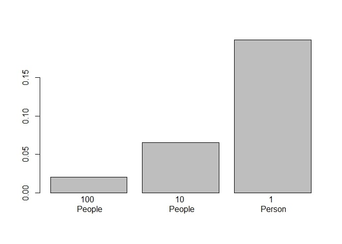
4. In the previous question, I wanted you to answer that with smaller sample sizes, we get larger variations in sample means. Now let us see if that is true through the method of simulation:

barplot(c(sd(sample_1), #sample of 100
sd(sample_2), #sample of 10
sd(sample_3)), #sample of 1
names.arg=c("100 \n People", "10 \n People", "1 \n Person"))

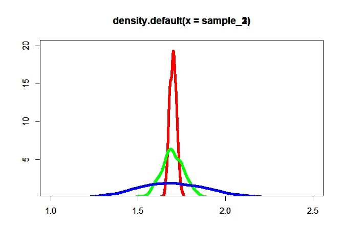
5) Another way of visualizing it:

d1 <- density(sample_1)
d2 <- density(sample_2)
d3 <- density(sample_3)
plot(d1, xlim=c(1, 2.5), ylim=c(1, 20), col ="red", xlab = "", ylab = "", lwd = 5)
par(new=TRUE)
plot(d2, xlim=c(1, 2.5), ylim=c(1, 20), col ="green", xlab = "", ylab = "", lwd = 5)
par(new=TRUE)
plot(d3, xlim=c(1, 2.5), ylim=c(1, 20), col ="blue", xlab = "", ylab = "", lwd = 5)

6. Explain what you see in both graphs. Why is it that larger samples yeald smaller standard deviations?

7. As we have seen in class, sample statistics have associated probability values, which are calculated according to its underlying population. Just think about it for a second. If you draw a random sample of 10 people from our original population, is it likely that you will see a sample mean of 2 meters? Why?

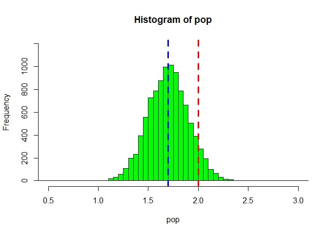
8. Let us visualize this. Run the code below. The red line indicates the number of samples (y axis) that got a mean of 2 when we randomly picked samples of 100 people from our original population.

hist(pop, col = 'green', xlim=c(0.5,3), breaks=seq(-50,50, 0.05), ylim=c(0,1200))
par(new=TRUE)
abline(v = 2, col="red", lwd=3, lty=2)
abline(v = 1.7, col="blue", lwd=3, lty=2)

9. Given everything you kow about the population and its sampling distributions, calculate the probability of getting a mean of 2 or more given that you draw a sample of 100 people.